
回归分析
### 回归分析研究的内容
- 确定Y与X1,X2…间的定量关系表达式。称之为回归方程
- 对求得的回归方程的可信度进行检验
- 判断自变量Xj对Y的有无影响
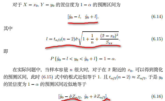
- 利用所求的的回归方程进行预测和控制
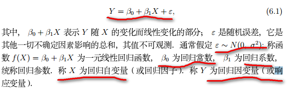
一元线性回归
一元线性回归方程:
σ^2 最小二乘估计: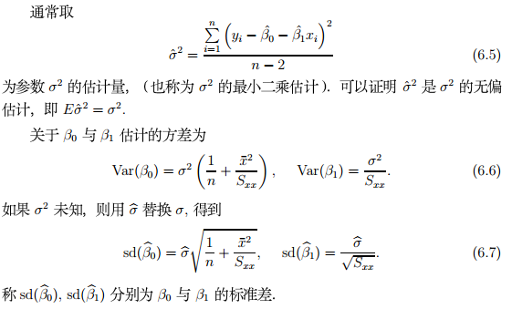
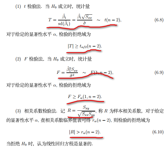
回归方程的显著性检验
假设检验: H0: β1 = 0, H1: β1 ≠ 0
通常采用三种方法来检验:
一元线性回归的简单例子:
	> x<-c(0.10,0.11,0.12,0.13,0.14,0.15,0.16,0.17,0.18,0.20,0.21,0.23)
	> y<-c(42.0,43.5,45.0,45.5,45.0,47.5,49.0,53.0,50.0,55.0,55.0,60.0)
	> result <- lm(y~ 1 + x) #表示y = β0 + β1*x + ε
	> summary(result) #用于提取模型的计算结果

	Call:
	lm(formula = y ~ 1 + x)

	Residuals: # 残差分布情况
	    Min      1Q  Median      3Q     Max
	-2.0431 -0.7056  0.1694  0.6633  2.2653

	Coefficients: #系数
	            Estimate Std. Error t value Pr(>|t|)
	(Intercept)   28.493#β0      1.580   18.04 5.88e-09 ***
	x            130.835#β1      9.683   13.51 9.50e-08 ***
	---
	Signif. codes:  0 ?**?0.001 ?*?0.01 ??0.05 ??0.1 ??1

	#残差标准差
	Residual standard error: 1.319 on 10 degrees of freedom
	# 相关系数平方
	Multiple R-squared:  0.9481,	Adjusted R-squared:  0.9429
	# F的统计量
	F-statistic: 182.6 on 1 and 10 DF,  p-value: 9.505e-08
参数β0和β1的区间估计:
	> x<-c(0.10,0.11,0.12,0.13,0.14,0.15,0.16,0.17,0.18,0.20,0.21,0.23)
	> y<-c(42.0,43.5,45.0,45.5,45.0,47.5,49.0,53.0,50.0,55.0,55.0,60.0)
	> result <- lm(y~ 1 + x)
	> interval <- function(fm, alpha = 0.05){
	+   A <- summary(fm)$coefficients
	+   df <- fm$df.residual
	+   left <- A[,1] - A[,2]*qt(1-alpha/2,df)
	+   right <- A[,1] + A[,2]*qt(1-alpha/2, df)
	+   rowname <- dimnames(A)[[1]]
	+   colname <- c("Estimate","Left","Right")
	+   matrix(c(A[,1],left, right), ncol = 3, dimnames = list(rowname, colname))
	+ }
	>
	> interval(result)
	             Estimate      Left     Right
	(Intercept)  28.49282  24.97279  32.01285
	x           130.83483 109.25892 152.41074
现在呢,我们可以利用我们算出的回归方程来进行预测。预测的结果由两部分组成,一个是预测值,另外一个预测区间。我们可以利用R提供的predict函数来进行预测。
	> x<-c(0.10,0.11,0.12,0.13,0.14,0.15,0.16,0.17,0.18,0.20,0.21,0.23)
	> y<-c(42.0,43.5,45.0,45.5,45.0,47.5,49.0,53.0,50.0,55.0,55.0,60.0)
	> result <- lm(y~ 1 + x)
	> newdata <- data.frame(x = 0.16)
	> predata <- predict(result, newdata, interval = "prediction", level = 0.95)
	> predata
	       fit      lwr      upr
	1 49.42639 46.36621 52.48657
实战一把:

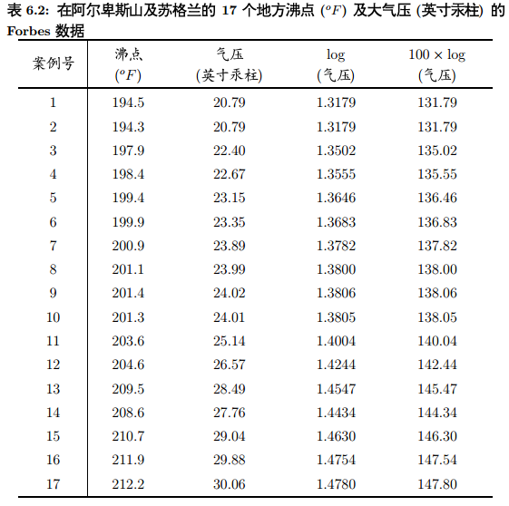
	> X<-matrix(c(
	+   194.5, 20.79, 1.3179, 131.79,
	+   194.3, 20.79, 1.3179, 131.79,
	+   197.9, 22.40, 1.3502, 135.02,
	+   198.4, 22.67, 1.3555, 135.55,
	+   199.4, 23.15, 1.3646, 136.46,
	+   199.9, 23.35, 1.3683, 136.83,
	+   200.9, 23.89, 1.3782, 137.82,
	+   201.1, 23.99, 1.3800, 138.00,
	+   201.4, 24.02, 1.3806, 138.06,
	+   201.3, 24.01, 1.3805, 138.05,
	+   203.6, 25.14, 1.4004, 140.04,
	+   204.6, 26.57, 1.4244, 142.44,
	+   209.5, 28.49, 1.4547, 145.47,
	+   208.6, 27.76, 1.4434, 144.34,
	+   210.7, 29.04, 1.4630, 146.30,
	+   211.9, 29.88, 1.4754, 147.54,
	+   212.2, 30.06, 1.4780, 147.80),
	+   ncol=4, byrow=T,
	+   dimnames = list(1:17, c("F", "h", "log", "log100")))
	>
	> forbes<-data.frame(X)
	> plot(forbes$F, forbes$log100) #看看在散点图上,两者有没有什么明显的关系
	>
	> result <- lm(forbes$log100 ~ forbes$F)
	> #看看线性回归方程的情况
	> summary(result)

	Call:
	lm(formula = forbes$log100 ~ forbes$F)

	Residuals:
	     Min       1Q   Median       3Q      Max
	-0.32261 -0.14530 -0.06750  0.02111  1.35924

	Coefficients:
	             Estimate Std. Error t value Pr(>|t|)
	(Intercept) -42.13087    3.33895  -12.62 2.17e-09 ***  #有很显著的差异了
	forbes$F      0.89546    0.01645   54.45  < 2e-16 ***
	---
	Signif. codes:  0 ?**?0.001 ?*?0.01 ??0.05 ??0.1 ??1

	Residual standard error: 0.3789 on 15 degrees of freedom
	Multiple R-squared:  0.995,	Adjusted R-squared:  0.9946
	F-statistic:  2965 on 1 and 15 DF,  p-value: < 2.2e-16

	> #两个参数的区间估计
	> interval(result)
	               Estimate        Left       Right
	(Intercept) -42.1308708 -49.2476789 -35.0140626
	forbes$F      0.8954625   0.8604095   0.9305155
	> #散点图和直线方程的拟合情况
	> abline(result)
	> #观察残差的情况
	> rr <- residuals(result)
	> plot(rr)
	> #发现第12个点有问题,那么要进行处理
	> text(12,rr[12],labels = 12, adj =1.2)
	>
	> result_new <- lm(forbes$log100 ~ forbes$F, subset = -12)
	> summary(result_new)

	Call:
	lm(formula = forbes$log100 ~ forbes$F, subset = -12)

	Residuals:
	     Min       1Q   Median       3Q      Max
	-0.21175 -0.06194  0.01590  0.09077  0.13042

	Coefficients:
	             Estimate Std. Error t value Pr(>|t|)
	(Intercept) -41.30180    1.00038  -41.29 5.01e-16 ***
	forbes$F      0.89096    0.00493  180.73  < 2e-16 ***
	---
	Signif. codes:  0 ?**?0.001 ?*?0.01 ??0.05 ??0.1 ??1

	Residual standard error: 0.1133 on 14 degrees of freedom
	Multiple R-squared:  0.9996,	Adjusted R-squared:  0.9995
	F-statistic: 3.266e+04 on 1 and 14 DF,  p-value: < 2.2e-16
总结:
一元线性回归求解的步骤: 1. 用plot看一下图形的情况,然后在写方程式 2. 对于求解出来的方程式进行验证,看看残差的情况,有没有异常的残差点。 3. 最后除去残差,重新计算方程式。
参考文献
1.《统计建模与R》
@This site is licensed under a Creative Commons Attribution-NonCommercial-ShareAlike 3.0 License@